For an ideal solution the entropy of mixing is assumed to be
where xA and xB are the mole fractions of the two components, and the enthalpy of mixing is zero,
The Gibbs free energy of mixing is therefore

The variation of these quantities is illustrated in the figure below.
Since mole fractions are always less than unity, the ln terms are always negative, and the entropy of mixing is always positive. The Gibbs free energy is always negative and becomes more negative as the temperature is increased.
For a regular solution the entropy of mixing is the same as for the ideal solution but the enthalpy now depends on composition,
where Β is the interaction parameter. The Gibbs free energy of mixing is therefore

The entropy of mixing of two ideal gases is identical to the formula assumed for the ideal mixing of liquids. It is derived as follows.
First we derive the entropy of expansion of an ideal gas. From the first and second laws
which can be rearranged to give
For an ideal gas PV = nRT and U does not change during a change in volume of the gas (no interactions). Hence, for one mole of gas,
and
If two pure gases A and B occupying volumes VA and VB are allowed to mix the new volume becomes VA +VB and each gas has increased its entropy by expanding into the space occupied by the other
The total entropy change is
The same formula can be obtained for equal size atoms in a solid lattice, but it cannot be derived for a liquid without very large assumptions. One such approach indicates the difficulties. The difference for liquids is that the volume available for each to expand into is only a proportion of the actual volume because the molecules themselves occupy a significant fraction of the volume. Thus the entropy of mixing of two liquids might be written
where VAf, etc. denotes the available free volume. To illustrate this difference the volume available to a water molecule in the liquid is about 0.03 nm3 (from the density). The radius of a water molecule is about 0.17 nm (OH bondlength + van der Waals radius of H), i.e. the actual volume of a water molecule (taken to be spherical) is about 0.02 nm3. The free volume is 0.01 nm3 and much smaller than the actual volume. It is also very difficult to estimate. We now make two assumptions. The first is that the fraction, f, of the molar volume that is free is the same for A as for B. Then

where φA and φB are the volume fractions. The second assumption is that VA = VB. Then φA is
and
The first assumption is very difficult to assess. There are situations where the second assumption is obviously wrong, for example for polymer solutions. These will be discussed later in the course.
The chemical potential is defined as
The chemical potential of a component of a mixture has two contributions,
one from the pure component, μo, and one from the mixing. The contribution from mixing is obtained as
follows.

which, after some manipulation, becomes
Hence
The chemical potential is the driving potential behind the transfer of matter between phases (or between chemical entities). It is comparable with temperature, which is the driving potential behind heat transfer, and with pressure, which drives volume changes. At equilibrium the temperature and pressure of different parts of the system must be equal. The same is true for the chemical potential. For a system with different chemical components A, B, etc. distributed between different phases, α, β, etc. the condition for equilibrium is that the chemical potential of component A must be the same in every phase, i.e.
with similar conditions for each of the other components.
Raoult's Law is obtained by equating the chemical potentials of solvent in solution and in the vapour. Using the subscript A to denote the solvent
The chemical potential of the vapour depends on the pressure of the vapour and can be written
The standard state of the vapour is when pA = 1, since that is when the ln term vanishes. It then depends on what units are chosen for pA. The convention is to use units of bar. The equations above give
When xA, i.e. for the pure substance, this equation becomes
where pAo is the vapour pressure of pure solvent, i.e.
A solution behaves ideally if it obeys Raoult's Law.
\textit{positive}.
The applet (adjustable diagram) shows how the vapour pressures of solvent and solute behave in a mixture ( Click here for notes about the use of java applets and click here for other physical chemistry applets). The diagram deals with the vapour pressures of ideal and regular solutions and can illustrate a wide range of situation. In an ideal solution there is no interaction and hence ideal behaviour is obtained by setting the Interaction Parameter to zero. When you do this you will see that the enthalpy of mixing is zero (left hand graph). TΔS and ΔG are also shown on the left hand side. When ΔH is zero the vapour pressures on the right hand side coincide with the ideal (black) values and conform to Raoult's Law over the whole composition range. Only for very similar pairs of liquids, e.g.dibromoethane and dibromopropane, is Raoult's Law obeyed over the whole range of mole fraction. In the common situation where it is not obeyed there are two types of behaviour, positive deviations, e.g. carbon disulphide and propanone, and negative deviations, e.g. trichloromethane and propanone. In these examples Raoult's Law is only obeyed where the solute concentration is low.
The standard examples showing (a) a strong positive deviation from Raoult's Law is acetone/carbon disulphide and (b)showing a stong negative deviation is acetone/chloroform. In the former the strong dispersion forces between the very polarizable sulphur atoms dominate and in the latter a weak hydrogen bond forms between the carbonyl group of acetone and the CH bond of chloroform.
A solution may be non-ideal either because ΔHmix is not zero or because ΔSmix does not have its ideal value. If there is a deviation from ideal behaviour the equation for the chemical potential must be modified to
where F(x) is the difference between the real and ideal chemical potentials. If F does not depend on concentration then it can be combined into the standard chemical potential, e.g.
This gives rise to the important Henry's Law standard chemical potential, which we will consider below. Usually F does depend on concentration and then it is convenient to express it in the form

where fA is called the activity coefficient, and we have omitted the concentration dependence, and aA is called the activity. The activity coefficient is a quantity that is determined by experiment. If we rederive Raoult's Law using the activity coefficient it is easy to see that Raoult's Law is modified to become
When this is compared with the ideal equation we have
and hence the activity coefficient can be determined experimentally. The equation shows that the observed pressure will be lower than the Raoult's Law pressure when the activity coefficient is less than unity. This occurs when F is negative, i.e. the chemical potential is less than its ideal value. This, in turn, will occur when the free energy of mixing is more negative than its ideal value (excess free energy of mixing negative) and the enthalpy of mixing is negative (interaction between A and B dominates those between A and A and between B and B).
The regular solution model is a quantitative explanation of non-ideal behaviour. The model assumes that the entropy of mixing is the same as ideal mixing but that the enthalpy of mixing is not zero. We now examine how a non-zero enthalpy of mixing might depend on concentration. Consider a mixture of A and B where A and B are randomly mixed and the average coordination number is z. If there are nB molecules of B in the mixture these will be in contact with a total of znB molecules, of which xAznB contacts are with molecules of A. This is the total number of BA contacts. Before mixing, these contacts would have been BB contacts in pure B and so the change in energy on mixing is, for the B molecules,
By the analogous argument the change in energy on mixing for the A molecules is
and the total energy change on mixing is
where we have also introduced a factor of 1/2 so as not to count all the interaction twice, and we have replaced z(2εAB − εAA − εBB)/2 by β, which is called the interaction parameter.
We make the approximation that the enthalpy of mixing is the same as the energy of mixing. The non-zero enthalpy (energy) of mixing now leads to an additional term in the chemical potential, μregular, which can be obtained by differentiating the enthalpy of mixing.
Hence the chemical potential of a regular solution is

where we have defined a new quantity, the activity coefficient, given by
A similar result is obtained for the activity coefficient of B.
The interaction energy clearly depends on concentration. However, before examining the concentration dependence we can see that the model explains the deviations from Raoult's Law. Designating the solvent as A, xA is approximately 1 at the Raoult's Law limit and xB is approximately 0. Hence BxA2 is approximately 0 and the chemical potential has its ideal value at the limit. Raoult's Law will therefore always approximate to the ideal limit.
Although Raoult's Law only works over the whole concentration range when the two compounds are almost identical, it generally also works well for the solvent in the region where the concentration of solute is low. However, even for relatively weak interactions, Raoult's Law cannot account for the vapour pressure of the minor component of the mixture, i.e. the variation of partial vapour pressure at the solute end of the plots. Although this region of the vapour pressure is not accounted for by Raoult's Law the variation of the vapour pressure of the solute is nevertheless linear over a limited range of composition (Henry's Law). Empirically, we can write
where p* is the hypothetical pressure reached when the mole fraction of solute is 1, rather than the saturated vapour pressure p0. We do not normally use a hypothetical pressure but write
which is Henry's Law.
The constant K is given by
Henry's Law requires that we replace the chemical potential of the pure substance with an empirical value
The difference between the Raoult and Henry behaviour can be explained qualitatively by considering what determines the chemical potential as the mole fraction of either A or B tends to zero. The two limiting situations are shown in the diagram below. In Henry's Law the solute molecule is surrounded by solvent molecules at the limit. In Raoult's Law the solvent molecule is surrounded by other solvent molecules. Thus, in Henry's Law it is the strength of the AB interaction (relative to AA and BB) that is significant, but in Raoult's Law it is only the AA interactions (or BB) that affect the behaviour.
At the Henry's Law limit the mole fraction of solute, xB is close to zero, xA is about 1 and the enthalpy term becomes approximately B. Thus there is an additional contribution of B to the ideal chemical potential. If the interaction is repulsive B is positive and vice versa. Henry's Law will only conform strictly with ideal behaviour when B is zero.
The applet above calculates the deviations from ideality using the regular solution model. It is capable of explaining a wide range of interactions. It is not always successful, however, one limitation being the enthalpy of mixing is quite often not symmetrical, in experimental systems, although it is so in the regular solution model. Another point to observe is that, when only dispersion forces are operative the energy εAB is less negative than the average of εAA and εBB with the result that B must be positive. This follows from the dependence of the dispersion forces on polarizability:
This is the reason that solutions of heavier species such as sulphur, bromine and iodine in organic solvents almost always show positive deviations. In observing how the vapour pressures respond to changes in the interaction parameter in the adjustable diagram above note that the behaviour becomes somewhat peculiar when the interaction parameter reaches its highest positive values. This is because the repulsion becomes so strong that it leads to phase separation.
When the interaction parameter β becomes sufficiently large and positive A and B will demix. The regular solution model can be used to predict the pattern of the phase separation of the two partially miscible components.
A quantitative model of the miscibility of two liquids is illustrated in the applet below. On the right is shown the phase diagram of two partially miscible liquids calulated according to the regular solution model. On the left are shown the three thermodynamic parameters. If the interaction parameter has a small positive value, the entropy of mixing ensures that the two liquids mix in more or less all proportions. As the interaction parameter increases so the entropy of mixing is less able to dominate the positive enthalpy of mixing and the free energy of mixing, although remaining negative overall, acquires a shape with two minima and one maximum. In the region between the two minima the free energy of the system is lowest if the system remains as two immiscible solutions with compositions corresponding to the two minima. This is because the free energy of such a phase separated system is represented by a horizontal line tangential to the two minima, whereas the free energy of the fully mixed system would follow the double minimum curve. The compositions of the two immiscible solutions are easily determined by finding the two minima in the free energy of mixing. This method has been used to calculate the phase diagram on the right hand side of the diagram below. As can be tested from the diagram the phase separation region widens as the interaction parameter becomes more repulsive and raising the temperature narrows it. There are some further points of interest. The dynamics of phases separation are driven by fluctuations. In general, if a fluctuation leads to a decrease in the free energy, it will happen spontaneously.In the diagram below there is a region coloured in pink where the variation of ΔG with a composition fluctuation is positive (examine the curvature of ΔG on the left hand side of the diagram). Spontaneous fluctuations in this region do not lead to phase separation. This makes the system metastable. The outer curve on the left then represents the true thermodynamic separation point and the inner curve, called the spinodal represents the end of the metastable region.
The compositions of the two phases in equilibrium in the above diagram and the value of the upper consolute temperature (the temperature at which the two solutions just become miscible) can be obtained by examining the properties of the differentials of the free energy of mixing. The compositions of the two immiscible phases are those corresponding to the two minima in ΔG, i.e. where the first derivative is zero and the second derivative is positive. The consolute temperature occurs at a point where both the first and second derivatives are zero, i.e. the plot has no curvature.
The regular Gibbs free energy of mixing is
Differentiating with respect to xA
This has two minima corresponding to the two immiscible phases in equilibrium and it has maximum at xA = 1/2. The equation for the minima cannot be solved analytically. However, further differentiation gives
This can be solved to give the upper consolute temperature as
The process of solution of a solid solute can be regarded as taking place in two steps. First the solute melts, which will involve a change in enthalpy, and then it dissolves, which is purely an entropic process in the ideal solution model. Because of the change in enthalpy the "ideal" solubility will be temperature dependent and an equation for this is derived as follows. We consider pure solute in equilibrium with solute in the solution, i.e. no solvent dissolves in the solid solute. Equating the chemical potential of the solute in the two phases gives
Rearranging and differentiating gives
Using the Gibbs-Helmholtz equation and applying it to the chemical potentials gives
This equation can be used as it stands but is more commonly used in its integrated form. Assuming the the enthalpy of fusion is independent of temperature gives
From this equation it can be seen that a plot of ln(solubility) against 1/T should give a straight line with a slope of -DH/T. Results are shown for the dissolution of naphthalene in several solvents below. The solubility of naphthalene is closest to ideal for solvents that are similar to it, e.g. benzene and toluene. There are two effects when the difference between solute and solvent increases; the slope of the plot changes, i.e. the apparent enthalpy of fusion is different, and the plot may become curved. The former results from the additional contribution of B to the enthalpy of fusion. The more repulsive the interaction between solute and solvent, the greater the apparent enthalpy of fusion and the steeper the solubility plot. This is why the slope of the graph is steepest for naphthalene in acetic acid. The curvature in the plot may arise because of deviation from ideality or because the enthalpy of fusion varies with temperature. In the derivation of the ideal solubility equation we have used the standard state appropriate to Raoult's Law whereas Henry's Law is more appropriate for the solute. It is this that causes the slopes in the figure to deviate far from the ideal value.
There are four other laws, the most important of which is osmotic pressure, which is dealt with separately when we come to polymers. The other three are depression of freezing point, elevation of boiling point and one governing the partition of a solute between two solvents. The principle is always the same, i.e. to start by equating the chemical potentials in the two phases of one of the components. Thus in the case of partition of a solute between two solvents we start by
The depression of freezing point concerns the depression of the melting point of the solvent by a small amount of solute dissolved (in the solvent only). The starting point is then
after which the derivation proceeds as for the temperature dependence of the solubility. The result is the following expression for the depression of freezing point
Depression of freezing point used to be used for the determination of molecular weights. Expressing the mole fraction x in terms of concentration gives the formula
The cryoscopic constant K is proportional to the molecular weight of the solvent and inversely proportional to its enthalpy of fusion. Thus CCl4 with Lfusion = 2.5 kJ mol−1 and M = 154 has a cryoscopic constant about 16 times that of water, for which Lfusion = 6 kJ mol−1 and M = 18.
The phenomena of depression of freezing point and elevation of boiling point are most clearly shown in the schematic diagram of chemical potential shown below. The chemical potentials of solid, liquid and vapour all decreases as the temperature increases. Phase changes occur at the intersections of the three lines because the system will always tend to jump to the state of lower chemical potential (with care it is however possible to maintain a system in the metastable supercooled, superheated, etc. state, i.e. water can be supercooled to about -40o C). The effect of adding a involatile solute, which does not dissolve in the solid, to the liquid is to lower its chemical potential by RTlnx. As shown on the digram this lowers the freezing point and raises the boiling point.
While the regular solution model is a much better aproximation than the ideal solution model it does not work for many liquids. This is most easily seen through the excess functions. These are defined as the difference between the actual free energy (enthalpy, entropy) and the ideal value. The regular solution model gives an enthalpy that is symmetrical with respect to composition, whereas it is often quite unsymmetrical. A particularly interesting pattern of behaviour is observed for mixtures of water with the lower alcohols. The Figure below shows the vapour pressures for ethanol/water, which show a positive deviation from Raoult's Law, and the corresponding excess functions. The explanation of this is quite subtle and has only recently been put on a firm experimental footing.
The interactions of an ethanol molecule with water are of two kinds. The OH group will interact strongly with H2O through hydrogen bonds. The ethyl group, however, interacts unfavourably because of the hydrophobic effect (see next section). That the hydrophobic effect dominates can be concluded from the unfavourable excess entropy of mixing. However, the unsymmetrical behaviour of the enthlpy of mixing suggests that the structure of the solution is changing with composition. Experiment (neutron diffraction) reveals that over much of the composition range the structure of alcohol/water solutions consist of interpenetrating networks of water and alcohol (bicontinuous structre). This is difficult to illustrate but a view (determined by computer simulation) is shown below. In these systems (from methanol to butanol), experiment shows that mixing is far from random. A better illustration of the type of structures involved in bicontinuous systems can be seen in a movie of the phase separation of two fluid colloidal phases on Dirk Aarts' website (Demixing in confinement). Hydrocarbons and water do not mix. Simple considerations of intermolecular forces suggest that they should (approximately, C and O are in the same row of the periodic table and the AA, BB and AB forces in their compounds should be equivalent). Experiments show that enthalpies of mixing of hydrocarbons and water are indeed slightly negative and hence favourable to mixing, but the entropies of mixing are not (the measurements for ethanol, which is not an extreme case, show this very clearly). There is not yet an agreed explanation of this effect, called the hydrophobic effect. The most widely used explanation is the following.
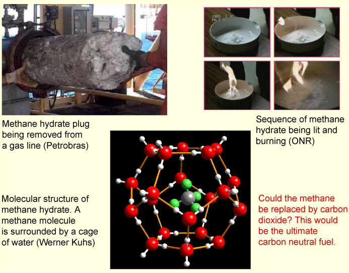
It is known that methane forms gas hydrates. There are such extensive deposits of one such hydrate over much of the northern hemisphere that the majority of the earth's stock of methane is in this form. Its appearance, properties and structure are illustrated in the picture below. The presence of the methane promotes an ordering of the hydrogen bonding in water that makes it solidify. Liquid water is an unusually open liquid and the restructuring allows some of its empty space to be occupied, which is energetically favourable. However, the ordering of the water results in a loss of entropy. It is argued that this is the reason for the unfavourable excess entropy of mixing that accompanies the hydrophobic effect. The problem with the explanation is that there is no direct experimental evidence for ordering in the liquid structure. It is therefore likely that the explanation lies more in the dynamics of the system than in the structure (see Dill & Bromberg, Chapter 30 for a good discussion of the hydrophobic effect).
Download regular.jar with RegSolnVPApplet.html and RegSolnMiscApplet.html for the two applets.

Temperature Dependence of Solubility
Other Ideal Solution Laws

Real Systems
The Hydrophobic Effect