Simple Solids and their Surfaces
The two main characteristics of a solid are that it has long range order and
that each atom is located in a particular position. The second property has the
consequence that, unlike the vapour or liquid phases, the particles of a solid
are "distinguishable". This will turn out to be very important in the
statistical thermodynamics of solids. However, the issue to be discussed here is
that of the long range order, how to describe it, how to detect it, and what
happens at a surface.
| Cubic Structures of Monatomic Systems
The structure of a solid is described as a combination of a
lattice and a repeating unit. The lattice is generated by
applying a set of symmetry operations to a point to generate an structure
that fills space. Note that these symmetry operations are different from
those with which you are already familiar for molecular point groups,
which do not generate infinite lattices. However, like the molecular point
group, there are only certain combinations of symmetry elements that
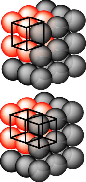
generate the infinite structures. The simplest representation of these
"space lattices" is in terms of their unit cells. On the right is shown a
cubic lattice of atoms and in the upper part the atoms making up the unit
cell are in red. The symmetry operations generate identical unit cells in
an infinite lattice. A second unit cell is marked in the lower part of the
diagram. The points of the unit cell are shown here as occupied by atoms,
but it is better to think of the lattice as consisting of a set of
points. |
|
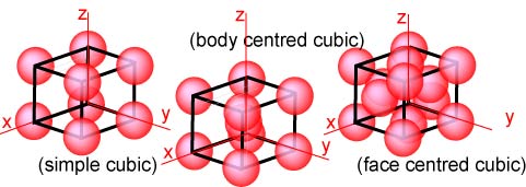
It is only necessary here to consider the cubic lattices, of which there are
just the three shown below. They have the obvious names simple, body
centred and face centred, but these derive from the more fundamental
symmetry conditions mentioned above. There are eleven others, of which one of
the most often mentioned is monoclinic, which is the lattice of lowest symmetry.
Once again the lattices below are represented in terms of atoms but are really
lattices of points.
For the determination of structures of solids and for considering the
structural characteristics of surfaces the arrangements of lattice points in
planes of the crystal are important. The different crystal planes are defined by
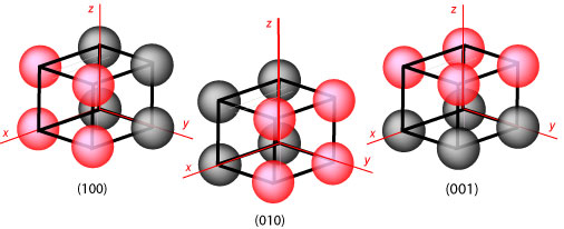
their Miller indices. The Miller indices of a crystal plane are
constructed by determining the intersection of the plane with the x,y,z axes and
then taking the reciprocals, by convention written as (hkl). In the
examples shown in the diagram below the intercepts of the plane of red atoms are
(1,∞,∞), (∞,1,∞) and (∞,∞,1) on going from left to right. Taking the reciprocals
of each intercept gives the Miller indices (100), (010) and (001) respectively.
Note that each Miller index represents a whole set of planes all parallel to one
another. Thus the expression (100) may be used to indicate either an individual
plane or the whole set of planes.
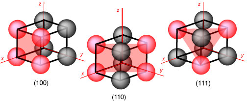
Within the simple cubic cell two other crystal planes are easily identified,
the (110) (there will be a set of planes of this type with different
orientations, of which the (101) and the (011) are the most obvious, but there
are additional ones with negative indices), and the (111). These two and the
(100) are the three sets of planes that are most important for basic surface
studies. The set is shown below with the atoms on the plane and the plane itself
marked in red
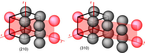
The planes so far shown are low index planes, but there are higher ones. The
way to evaluate the indices of these planes requires a slight alteration in the
procedure. The intercepts of the plane on the xyz axes are all scaled down by
the factor that reduces the highest intercept (other than ∞!) to 1. The diagram
below shows the (210) and (310) planes. In the former the intercepts are the set
(1,2,∞). These are multiplied by 1/2 and the reciprocals then give (210).
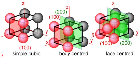
For the three cubic structures the structural arrangement within a plane and
between different planes may be different. Below are shown the (100) planes of
simple, body centred and face centred cubic lattices. In the body centred and
face centred cubic structures there are planes of atoms (marked in green)
interleaving the (100) planes. These, together with the (100) planes, make up
the (200) set of planes (intercepts (�,∞,∞).
Structures of Surfaces of Bulk Cubic Structures
The lattice
parameter of a cubic lattice is simply the length of the cube edge and here
is denoted as a. If a were the same for the three cubic lattices,
the atomic density would be greatest for face centred and least for simple
cubic. When a crystal is cut to reveal a particular crystal plane as surface the
surface structure is easily calculated from the lattice parameter and the
lattice, assuming that it does not alter (reconstruct). The surface will
be referred to as an (hkl) surface. However, when surface experiments are
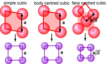
being considered, it is easier to use a surface lattice for reference. As an
example, the (100) surfaces of the three cubic structures are redrawn again
below and the resulting surface lattices shown in purple. Those of the simple
and body centred lattices are identical and are square lattices of lattice
parameter a. That of the face centred lattice is also square but of
spacing a/√2. Thus, the (100) planes of all three cubic lattices give
surface lattices of identical symmetry, i.e. simple square lattices. When
these have the original symmetry of the crystal plane of the solid they are
designated (1x1) lattices. This each one of the surface lattices below is a
(1x1) lattice. The purpose of this simple, but incomplete description will be
made clearer below.
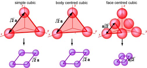
The diagram below shows the surface lattices obtained from a cut along a
(111) plane of each of the cubic lattices. The resulting lattice parameter of
the surface lattice is given in terms of the parameter of the original cubic
lattice. The same simple haxagonal lattice symmetry is again obtained for all
three cubic structures and again the three lattices are all designated (1x1),
although they are now completely different from the (1x1) lattices obtained from
a (100) plane of the bulk crystal. The complete description of a surface lattice
must therefore include the indices of the plane of the original crystal.
|
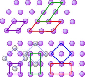
Although a surface may be cleaved to generate a particular surface, it
usually rearranges to some extent. Sometimes this is just that the
distance between the surface plane and the adjacent one underneath is
slightly different from the bulk value. Less oftenly, the symmetry of the
surface plane changes fundamentally. How this works is shown for both
(111) and (100) surfaces alongside. In each case the (1x1) lattice is
shown in purple, (2�1) and (1�2) are shown in red and green, and a
(√2�√2)R450 is shown in blue. The numbers denote
the lengths of the sides of the new lattice relative to the (1�1) and the
R450 indicates that the lattice is rotated
through 450 relative to the original. Note that a further ambiguity in the description of the surface lattice
as a multiple of the basic (1�1) lattice is that it does not specify where
the lattice is. Thus any of the alternative reconstructed lattices
indicated by the black/grey atoms is a
(√2�√2)R450 lattice.
|
|
Finally, note that the lattices of adsorbed layers of gases are treated
in exactly the same way as the reconstructed surfaces. Thus, the ambiguity
associated with the (√2�√2)R450 lattice in the
figure above applies equally to adsorbed layers, e.g. an
adsorbed layer of hydrogen atoms. This is important and will be returned
to below.
Diffraction from Crystalline Solids
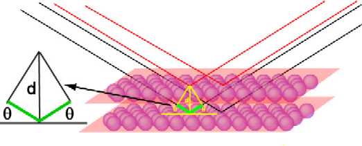
The figure below represents the scattering of radiation from two crystal
planes of a solid. The red and black lines represent radiation reflected from
the upper and lower set of planes respectively. The reflection is treated as
though the two planes of atoms behaved like half-reflecting mirrors. There is a
difference of 2dsinθ in the pathlength travelled by the two beams
of radiation where d is the perpendicular distance between the planes
(the path difference is marked in green and the expanded construction alongside
makes the geometry more clear). As the angle of reflection is changed so does
the difference in pathlength travelled by the two beams. When the path
difference is equal to an integer number of wavelengths the two beams will
reinforce one another and when it is an integral number of half wavelengths the
two waves will interfere destructively with one another. The intensity of the
total reflected radiation will vary sinusoidally with θ. However, if
reflection is from a large set of parallel planes the interference builds up so
that it is destructive at all angles except those satisfying the constructive
interference condition, i.e. when θ is given by
nλ = 2dsinθ
This is Bragg's law. The
method of deriving it here is somewhat unsatisfactory but the alternatives would
require more effort than you need to put in.
Although the physical model of diffraction given by the Bragg's law approach
is not a good one, the law itself is correct. Thus, the (100) planes of a simple
cubic structure will give diffraction peaks when
sinθ = nλ/2a, n = 1, 2, 3, ..
where a is the lattice parameter. An alternative way of stating this
is to say that there is diffraction from the (100), (200), (300), .. planes at
sinθ = λ/2d, d = a,
a/2, a/3, ..
The two statements are equivalent, but the second
is much more commonly used. Since Bragg's Law applies to all sets of crystal
planes the lattice can be deduced from the diffraction pattern, making use of
general expressions for the spacing of the planes in terms of their Miller
indices. For cubic structures
d(hkl) =
a/(h2 +
k2 +
l2)1/2
Note that the smaller the spacing the higher the angle of diffraction,
i.e. the spacing of peaks in the diffraction pattern is inversely
proportional to the spacing of the planes in the lattice. The diffraction
pattern will reflect the symmetry properties of the lattice. A simple example is
the difference between the series of (n00) reflections for a simple cubic
and a body centred cubic lattice. For the simple cubic lattice, all values of
n will give Bragg peaks. However, for the body centred cubic lattice the
(100) planes are interleaved by an equivalent set at the halfway position. At
the angle where Bragg's Law would give the (100) reflection the interleaved
planes will give a reflection exactly out of phase with that from the primary
planes, which will exactly cancel the signal. There is no signal from
(n00) planes with odd values of n. This kind of argument leads to
rules for identifying the lattice symmetry from "missing" reflections, which are
often quite simple.
Electron Diffraction from Surfaces
Electrons are the preferred radiation for doing diffraction from surfaces
because they are so strongly scattered by atoms that the scattering is almost
exclusively from the surface layer. The positions of peaks in the diffraction
pattern are determined by Bragg's Law, just as for x-ray or neutron diffraction
from 3-D solids (at this stage you should not worry about the fact that it is
not easy to see how Bragg's Law could be logically derived for a surface layer).
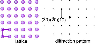
The (100) surface of a cubic solid is shown below with its diffraction pattern.
Because there is a Bragg peak for every set of planes it is not difficult to
work out that the diffraction pattern has the same symmetry as the original
lattice, although the intensities of the peaks fall off away from the origin for
reasons that will be discussed below (the large central spot in the diffraction
pattern is from the direct electron beam, which is usually in normal incidence
on the surface). Some of the Bragg reflections are designated by the Miller
indices of the planes (or lines for a 2D lattice) of atoms they come from. Thus
the series (10), (20), (30) cam be regarded as the n = 1, 2 or 3
reflections from the (10) plane or reflections from the (10), (20) or (30) sets
of "planes". Planes can have positive or negative Miller indices, so the
diffraction pattern is symmetrical about its centre.
|
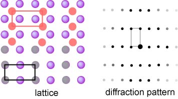
The spacing of the reflections is inversely proportional to the
separation of the planes and this is illustrated by the (2x1) lattice
alongside and the corresponding "(1x2)" symmetry of the resulting
diffraction pattern. It is important to note that the positions of the
Bragg peaks only give the symmetry of the lattice. They do not distinguish
between the grey and orange lattices, which would give identical
diffraction patterns. |
|
Finally, an optical analogue of LEED is demonstrated in the applet below. Although the pattern shown on the right is the result (exact) of light passing through a set of apertures shown on the left, the outcome is identical with that reflected from a set of apertures, i.e. done in the same geometry as a LEED experiment. All the simple conclusions from the paragraph above can be demonstrated, as well as the more complicated issues associated with the effect of the shape of the individual objects on the intensities. However, since the calculated pattern is only for a limited number of objects, effects of the finite size of the array can also be seen. These can be minimized by setting the number of horixontal and vertical slits to the maximum valur of 11 and mainly take the form of additional features in between the main diffraction spots. This calculation is a large one and may be quite slow. It may therefore be worth downloading it. (Applet is in "twoD.jar" and controlling program is "TwoDAppletJ.html". Setting the parameter "alias" to 1 introduces aliasing, which greatly improves the quality of the picture but uses more computer power.)
Intensities in Diffraction
All the discussion so far has been only of the lattice and the positions of diffraction peaks. Although this is what you most need to understand for the purposes of LEED and surfaces, it is only the first step in determining structure using diffraction methods. The lattice symmetry is determined by the positions of the the diffraction peaks but structure is determined from the intensities of the diffraction spots (or peaks). Only a very brief outline is given here.
|
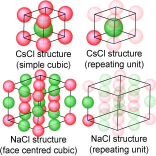
Associated with each point of the lattice is a repeating unit. The structure of the solid is generated by combining this unit with the repeat structure of the lattice. Two examples are given alongside. One is the CsCl structure (Cs+ in red, Cl− in green) which is simple cubic (it is often mistakenly identified by students as body centred) and the repeating unit is a single CsCl with the configuration shown on the right. The whole structure can be generated by placing this unit at each of the lattice points of the simple cubic structure. The second example is NaCl, whose lattice is face centred cubic and once again the repeating unit is a single NaCl, but now oriented differently with respect to the lattice. (There are other possible choices for the repeating NaCl unit.)
|
|
The first step in calculating the intensity is to sum the scattering from each of the atoms in the repeating unit but in the framework of the particular Bragg reflection being considered. For example, for the (100) reflection of CsCl, the scattering of the Cl− is exactly out of phase with that from the Cs+ because it occurs exactly halfway between the (100) planes. Hence the contribution of the repeating unit to the amplitude of the scattering is fCs − fCl. (Note that if the atoms were identical, as in a true body centred cubic structure, this amplitude would be zero.) The intensity of the (100) peak is just the square of this amplitude. For the (200) peak the amplitude (usually called the structure factor) would be fCs + fCl. These are trivial examples and it is evident that, if the repeating unit is a complex organic molecule (or several molecules) or a protein, that the calculations become very complex.
The relation of intensity to structure relies on the radiation only being scattered once. It is quite easy to realize that if the rays used in the Bragg reflection construction were scattered twice or more (multiple scattering), the geometrical relationships between them would be difficult to work out. The chances of multiple scattering occurring increase rapidly, the more strongly the radiation is scattered. The whole sensitive of LEED to surfaces is based on very strong scattering. Hence, it is very difficult to calculate structure from the intensities in LEED patterns and this is why a simple analysis does not, for example, reveal where a lattice of adsorbed atoms lies in relation to the underlying substrate. However, methods now exist, using long computations, that are able to determined structure from LEED in many cases.