Liquids and Solutions: 2nd Year Michaelmas Term: Introduction
Liquids, Solids and Gases
The density of a liquid is only slightly different from that of the corresponding solid and hence the mean separation of the molecules must be comparable in the two states. The fundamental differences between the crystalline solid and liquid states is that there is long range order in the crystalline solid but there can only be local order in the liquid. Amorphous solids (e.g. ordinary glass) also have no long range order and there is little difference between the structures of liquids and amorphous solids. They can, however, be distinguished by the time scale of the motion. In a liquid a molecule explores the whole space occupied by the liquid in a relatively short time whereas the movement between adjacent positions in amorphous solids is more or less infinitely slow. For the purposes of assessing the role of molecular interactions on the nature of solids, liquids and gases, it is important to have a common means of describing their structures.
The Radial Distribution Function
The rapid molecular motion in a liquid and its lack of long range order make it difficult to describe. The function that is used to describe the average structure is the radial distribution function, usually written g(r). To construct g(r) we start by taking an instantaneous snapshot of liquid, as shown in a 2-D representation in the diagram alongside. With reference to the purple coloured molecule there are two groups of molecules, one whose centres are at a distance of about a molecular diameter from that of the reference molecule (green) and one whose centres are at about two molecular diameters (pink). The range of distances between the reference molecule and the molecules in the first coordination shell is much narrower than for the second coordination shell.
Taking the centre of the purple reference molecule as being at r = 0 we construct a histogram of the molecules at a given distance r from the reference molecule. A typical result would be as shown in the second diagram (distances correspond approximately to liquid argon). The first coordination shell gives rise to a noticeable cluster whereas the second coordination shell is more diffuse, and it becomes difficult to discern a pattern for subsequent coordination shells. We now repeat this process for every other molecule in the liquid, taking as reference molecules A, B, C, D, etc. for the same instantaneous snapshot (see figure below). Each gives a slightly different histogram. Finally we average the results of all the histograms. The resulting plot, shown below right for liquid argon at its triple point, gives the probability of finding a molecule at a given distance from any chosen central reference molecule.
A more convenient way of representing the structure of the liquid is to remove the 4πr2 factor from argon (A) to obtain the radially averaged number density distribution, argon (B). The radial distribution function, argon (C) or g(r), is obtained by dividing argon (B) by the bulk number density, nbulk. This distribution function has the simplifying feature that it tends to unity at large r.
The qualitative appearance of radial distribution functions for monatomic liquids is similar. There is an obvious first coordination shell and some indication of at least a second coordination shell. However, molecules (as distinct from atoms) may have g(r) of more complex appearance. On the right are shown the g(r) for solid and liquid sulphur. Sulphur forms crown-shaped, covalently bonded S8 rings in both solid and liquid states. The well-defined molecular structure of the S8 molecules gives rise to a sharp peak at 0.206 nm (the S-S distance in the ring). In the solid state the peak in g(r) corresponds to precisely two nearest neighbours. When sulphur melts the ring structure persists but there is some bond breaking, which causes the intramolecular peak at 0.206 nm to drop slightly in intensity (1.7 nearest neighbours). A small new peak also appears at 0.27 nm. The longer range structure that is present in g(r) for the solid is also largely washed out in the liquid.
The difference in average structure between a solid and a liquid can be illustrated by consideration of the structures of liquid and solid argon at coexistence, as shown by the g(r) in the diagram above on the left. For the solid the atom positions have been taken to be those for a face centred cubic lattice but with a significant amplitude of vibration. The number of atoms in the first coordination shell is about the same in liquid and solid (exactly 12 in the solid) but the two structures become quite different after the first coordination shell. The difference in average structure between a gas and a liquid can also be illustrated in terms of the radial distribution functions, as shown on the right. The liquid g(r) is shown in black and the g(r) for the gas is shown at two temperatures, 90 K (in red) and 300 K (in green). At first glance there appears to be more correlation in the gaseous state than might be expected. However, it must be remembered that g(r) is normalized to a density of unity. The gas phase density is very low and so, although there is a large peak in g(r) at 90 K, the absolute number of atoms clustered around the central reference atom is minute.
The next diagram is a java applet that allows us to play around with some of the above ideas introduced above ( click here for notes about the use of java applets and click here for other physical chemistry applets). The diagram is a real time molecular dynamics simulation of a set of interacting particles in two dimensions. The program is a simplified version of one written by David Wolff (the original can be viewed directly at his website). The version here is simplified in order to illustrate the key points. You do not need to understand the technicalities of the simulation in detail but there are some points that you should appreciate in order to be convinced by the results. These are, in greatly simplified form:
(i) The atoms are initially placed in a regular lattice (Reset button). They are given an initial displacement (Start). The forces acting on each atom in the ensemble are then computed and the resulting motion or change in motion calculated for each atom by solving the equations of motion. After a short time step, the new positions are calculated, then the new forces and the change in motion, etc. The system is taken to be at equilirium when the initial impulse is dissipated throughout the system and the temperature (or energy) of the ensemble is reasonably stable (this can be monitored by selecting the energy to be displayed in the graph at the bottom).
(ii) The procedure that is used to avoid any effect of confinement is that when an atom leaves the box, it is replaced by an atom coming in from the opposite side of the box with the same velocity (periodic boundary conditions). This minimises the effects of confinement on the dynamics, although it does affect the display.
(iii) The interaction potential is a realistic one and includes the finite size of the atoms and an accurate representation of the intermolecular attraction. The calculation is set for argon.
You should play around with the simulation to explore the radial distribution function in different situations and to try to ascertain the factors that underly the existence of solid, liquid and gaseous phases. The following are some suggestions:
(i) Set the density to its maximum value and press the reset button. This shows the regular lattice used as the starting point. Start the simulation and convince yourself that there is no temperature at which this solid will melt. Although the vibrational motion in the lattice becomes more vigorous at the highest temperature, the regularity of the lattice structure is maintained. This is best monitored by choosing to look at the radial distribution function. At all temperatures it consists of discrete peaks, as described in the introduction, although the peaks do broaden as the temperature increases.for the calculation.
(ii) With the simulation still running, gradually decrease the density until the solid melts (note that density changes on the display are shown by scaling the atom size to a changing box size). You can monitor melting in part through the radial distribution function and in part by watching one atom and seeing when it is displaced from one "lattice position" to another. Play around with different combinations of temperature and density. The liquid state is distinguished by the atoms becoming delocalised (they will in time sample the whole space) and by the radial distribution function being non-zero at all points greater than the core radius.Unfortunately the size of the box is not large enough to see the convergence of g(r) to unity.
(iii) Lower the density to its minimum value and gently increase the temperature to its maximum value (gently, because a sudden change in time step and energy may generate a configuration where the cores of two atoms overlap and then the energy of the system jumps to unmanageable values; if this happens, just press reset). You will now see typical gas phase motion of the atoms, although the density is a lot higher than a typical gas. The radial distribution function under these conditions is as described in the introduction. There is an exclusion zone corresponding to the hard cores and a slight maximum at distances beyond this where the attraction between the molecules causes them to undergo sticky collisions.
(iv) With the density at its minimum lower the temperature and you will see that the atoms start to form small clusters (this takes some time). On the limited scale of the simulation this is condensation to form drops of liquid. It makes it clear that the attractive forces are responsible for the formation of the liquid state. These clusters would not form if the potential were purely repulsive.
(v) Finally reexamine the transition between solid and liquid, convincing yourself that the attractive forces only play a very minor role in this transition, which can be approximately described as occurring when the vibrational amplitude is large enough to displace an atom from one lattice position to the adjacent one.
Experimental Determination of the Radial Distribution Function
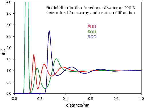
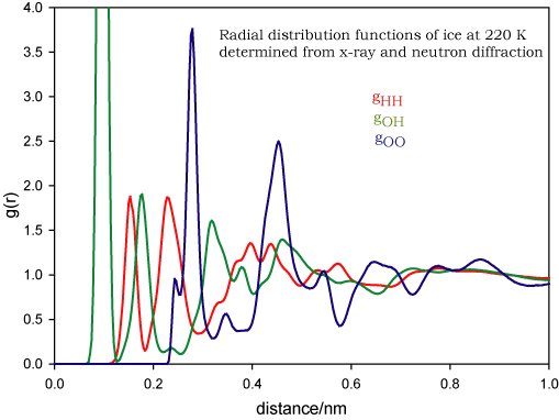
The radial distribution function is not only a means of describing liquid structure but it is the function most readily accessible from experiment. The x-ray or neutron diffraction of a monatomic liquid is related by a one-step mathematical transformation to the radial distribution function (by a Fourier transform). Note that the diffraction patterns of solids are normally analysed in a completely different way (see simple solids and diffraction), although they can also be analysed in the "liquid" way. The situation is more complicated for liquids containing more than two atoms. Consider water. The complete description in terms of radial distribution functions requires three radial distribution functions, gHH, gOH and gOO. The transformation of the x-ray diffraction pattern of liquid water will give a mix of these and they cannot be disentangled. However, the contribution of H and O to the neutron diffraction pattern is different from that in x-rays and this represent a second independent measure. This is still not enough to determine three radial distribution functions. However, H and D are scattered differently by neutrons and so the diffraction pattern of D2O can be used as the third independent piece of information. Thus the three radial distribution functions of water are experimentally accessible. They are also very interesting and are shown below for water and ice (N.B. these are experimentally determined and have been tabulated by A.Soper and can be found on the ISIS database). You should examine these two diagrams very carefully and make sure that you can match them to the picture of water structure that you are familiar with.
.
.
Radial Distribution Functions and Mixtures
A qualitative feel for some of the main issues to do with mixing can be obtained from the quantitative model shown below. This is a Monte Carlo simulation of a 2D version of something called the Ising model.
The applet allows you to do your own simulations. It demonstrates mixing on a lattice and, although the model is derived from a model to describe magnetic interactions, the mathematics is appropriate to the mixing of two liquids. Some suggestions for simulations are outlined below the diagram.
As set up here the program simulates the mixing and demixing of two liquids A and B on a square lattice. There are two adjustable parameters, the temperature and an interaction parameter, which is a measure of the interaction energy between A and B. The starting lattice configuration can be chosen to be either the separated liquids A and B or the perfectly ordered mixture. The former corresponds to the low temperature limit of strong repulsion between A and B and the latter to the low temperature limit of strong attraction between them. You can switch between the different starting points by toggling the Reset Button. The method used for the simulation is the Monte Carlo method, which is completely different from that used for the simulation shown in the section on the Radial Distribution Function. The following section in italics, which you do not need to understand, outlines the method. The subsequent paragraph suggests some simulations that you might perform.
An equal number of A and B "atoms" is displayed initially on a square lattice, each atom having four nearest neighbours. One of these, chosen at random, has its identity reversed (B becomes A or vice versa). The resulting change in energy and the corresponding Boltzmann factor (exp(−ΔE/RT)) are computed. If the Boltzmann factor is greater than a random number between 0 and 1 the change is accepted, if not it is rejected (i.e. decreases in energy are automatically accepted, increases in energy are accepted with decreasing probability as they become larger). The procedure is then repeated as long as required. The weighting of the choice of configurations towards those that are energetically more favourable ensures that the system reaches equilibrium much more efficiently than would be achieved with purely random changes. The method is known as the Monte Carlo method, it is exceedingly widely used for the solution of problems of this type, and the code used here can be found in Chandler: Introduction to Modern Statistical Mechanics, Oxford, 1987, pp 184-5. Note that periodic boundary conditions are used, as in the simulation shown earlier, to minimize the effects of the boundaries. It may seem from the operation of the program here that multiple changes are being implemented. This is not the case but, since the display is the slow part of the simulation, it is only being updated after every 20 successful moves.
The following are suggestions for some basic simulations.
(i) Before starting the program, set the B slider to 0. This corresponds to zero interaction between A and B, i/e/ to an "ideal" system. Start the program. The system very rapidly mixes, i.e. at the minimum temperature of 150 K the system will mix. Note that this occurs even though there is no net interaction between A and B. The interactions AA, BB and BB are all equal. This is ideal mixing. What would be the differences in the radial distribution functions gAA, gBB and gAB?
(ii) Reset the system to start with the separate A and B phases and start the simulation keeping both sliders in their initial positions (lowest temperature and maximum attraction) and confirm that the system equilibrates to the "chessboard" configuration as expected. When the system seems reasonably stable change the interaction parameter to zero and allow the simulation to run for a while. Note that the appearance is not the same as with B = -2000 J mol−1. Increase the interaction parameter to +2000 J mol−1 and, again, allow the simulation to run for a while. What happens? Note also how it happens. The large clusters grow at the expense of the small clusters. Now increase the temperature to its maximum value and again wait to see what happens.
(iii) Repeat the above but starting from the initial chessboard or mixed congiguration using the reset button.
(v) Start the simulation from the phase separated condition with the energy set to maximum repulsion, i.e. slider to the right, but at the lowest temperature. The system remains phase separated, although there are significant fluctuations at the two interfaces. Increase the temperature gradually and observe the amplitude of these fluctuations increase. Can you suggest a reason for the fluctuations? Continue to increase the temperature and estimate the point at which mixing is complete. Then decrease the temperature and test the extent to which you can reverse the process. The phase separation is reversible but it is difficult (not impossible) to recover the initial positioning of the to separated phases. If you try this you will find that it is the periodic boundary conditions that are the main obstacle.
The applet introduces the two main models of liquid mixtures, ideal solutions and regular solutions. In the ideal solution there is no energy of interaction. Mixing is driven by the temperature independent entropy of mixing or the temperature dependent Gibbs free energy of mixing. The regular solution assumes the same entropy of mixing as the ideal solution but it includes a model for the enthalpy of interaction. If the enthalpy of mixing is positive it may be sufficient to offset the free energy of mixing coming from the entropy of mixing and to maintain or bring about phase separation. However, it also has a strong effect on the energy of binding a molecule, whether or not there is phase separation, and this manifests itself on the thermodynamic properties of the system. This is dealt with quantitatively in the next lecture.
 .
.
 .
.