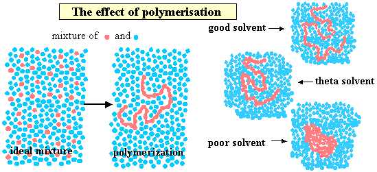
A polymer is generated by joining many monomers together. To show some of the consequences of such a connected structure we use the same simple model that we used to introduce amphiphiles, i.e. chemical groupings with opposing solubility characteristics are represented by different shapes (squares and circles) but those with similar characteristics are represented with different colours but the same shape. The figure below shows one type of circle dissolved in another but with the difference that one sequence of circles is joined to form a polymer. In comparison with free circles, which would form an ideal solution, the movements of the segments of the polymer are restricted and the motion of the polymer molecule in solution is then relatively complex, consisting of changes in conformation with some translational movement of the polymer as a whole. Polymerisation must therefore lead to substantial differences in the solution behaviour. One difference is that any unfavourable interaction of the monomer unit with the solvent is magnified by the large number of such interactions for each polymer molecule. Since dissimilarity generally leads to a positive enthalpy of mixing this means that the polymer only dissolves in a solvent with which its monomer is similar (i.e. circles in circles). The right hand side of the figure shows what happens to the polymer dimensions as the "quality" of the solvent is varied from poor (polymer solubility reduced), through the q condition (where there is no nett effect of solvent on the polymer dimensions) to good. The full range of behaviour illustrated can often occur over a few tens of K or by varying the composition of a mixed solvent over a small composition range.

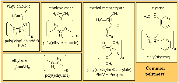
There are many types of polymer, the simplest being a linear connection of one chemical species to form a homopolymer, of which several examples are given in the panel below. Copolymers involve more than one chemical species and they can be combined in a variety of ways, e.g. alternating, randomly or in blocks. There are also non-linear combinations, e.g. star, comb, dendritic, etc. The selective use of these structural possibilities leads to a wide range of technological applications of polymeric materials.
The simplest model of a polymer structure is the three dimensional random walk (random flight). The applet below ( click here for notes about the use of java applets and click here for other physical chemistry applets; the relevant filenames for the polymer applet are randWalk.jar and RandomWalkAppletJ.html) calculates a new one thousand step random walk each time the button is pressed. The end to end distance is given together with its cumulative average.
The polymer consists, at start-up, of 1000 segments of length unity and these are free to rotate through any angle with respect to adjacent segments (random flight model, three dimensional random walk model). The polymer is drawn in perspective to capture the 3-D structure. The two ends of the polymer are marked with black rings. The brighter coloured, larger segments are in the foreground and the paler, smaller segments are furthest away. On pressing New random walk a new configuration is generated. The right hand side shows the square root of the end-to-end distance of the configuration shown and the accumulated root mean square end-to-end distance. It also plots a histogram of the accumulated RMS end-to-end distances. There is one adjustable parameter, which is discussed further below.
You should try the following.
(i) Repeat the calculation enought times to generate a reasonably stable histogram of RMS end-to-end distances. Note the very wide variety of possible configurations, the quite wide distribution of RMS end-to-end distances in the histogram, and the large number of 'data' you have to accumulate to generate a representative distribution. Note also that there is a most probable RMS end-to-end distance and that this is the square root of the fully extended length of the polymer, i.e. 10001/2. Since this end-to-end distance is the most probable, it is the one for which the entropy has its highest value.
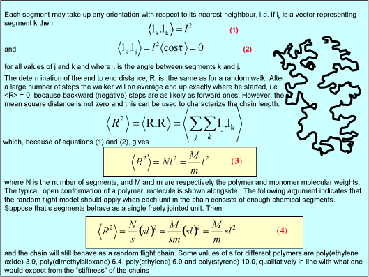
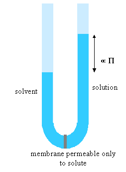
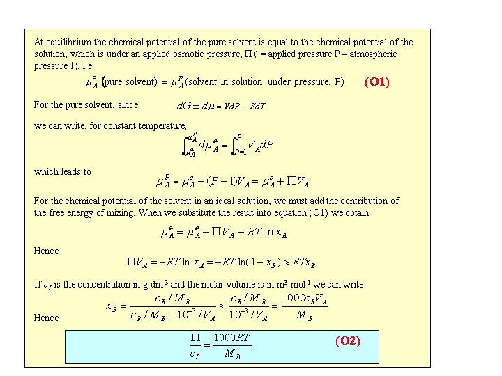
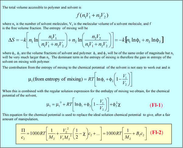
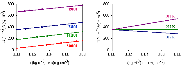
(ii) The lever changes the polymer as follows. It incorporates a number of the initial segments into a single segment (changes the persistence length) and correspondingly reduces the number of segments, thus increasing the length of an individual segment while keeping the fully extended length of the polymer constant. Set the value of the slider to a segment length of 2. Press restart to restrt the calculation of the histogram. You will notice that the values of the RMS end-to-end distance increase (the scales in the left hand graph have been kept as the original segment length of unity). Repeat the calculation until you have a representative histogram and compare the RMS end-to-end distances for segment lengths 1 and 2. The ratio should be 1.4 (21/2). The applet does the calculation numerically but the RMS end-to-end distance can also be related to the molecular weight and the length of the individual segments analyticlly as in the panel below. The random flight model only seems unrealistic if one makes the mistake of assuming that a random flight segment is the same as a chemical segment. For each homopolymer the number of chemical segments needed to produce a segment that follows the random flight model varies according to the stiffness of the structure and some values are given for common polymers at the bottom of the panel below. This is essentially the calculation (ii) that you made for the applet above. Osmotic pressure is the most useful of the colligative properties (depression of freezing point, etc.). It is widely used for the determination of molecular weights of large molecules such as polymers and proteins. The principle is shown in the diagram below. The pure solvent and solution are separated by a membrane permeable only to the small solvent molecules (the polymer cannot pass through). The chemical potential of the solvent is lower in the solution and it will therefore tend to pass through the membrane from pure solvent to solution. This process can be opposed by applying a pressure (additional to atmospheric and called the osmotic pressure) to the solution. The relationship of the osmotic pressure to the concentration and molecular weight of the solute is derived in the panel below the diagram. The thermodynamic properties of a polymer in solution are important in the determination of the molecular weight by osmotic pressure. Because a polymer is very large in comparison with the solvent molecule the entropy of mixing does not take on the simple form that it has in an ideal solution. As written in the panel below, the mole fractions in the expression for the ideal entropy of mixing must be replaced by volume fractions. There is also a contribution to the free energy of mixing from the enthalpy of mixing of polymer and solvent. Any small enthalpic interaction between a polymer segment and a solvent has to be multiplied by the number of segments. Thus, even small interactions become significant. The calculation of the enthalpy of mixing is similar to that used in the regular solution model except that volume fractions are used instead of mole fractions. The panel below summarizes the two contributions (first derived by Flory and Huggins, and often known as the Flory-Huggins model) and substitutes the resulting chemical potential of the solvent into the derivation of the osmotic pressure to give the important equation (Fl-2). Comparison of the ideal and non-ideal expressions for the chemical potential shows that B contains one contribution from the excess entropy of mixing (the 1/2 term in equation (Fl-2)) and one from the excess enthalpy of mixing (the c term). Taking the enthalpy of mixing to be zero leads to a positive value of B, resulting from the positive excess entropy of mixing. The positive excess entropy of mixing creates an additional driving force for diluting the solution with solvent, i.e. a higher osmotic pressure than would be expected from ideal behaviour. The enthalpy of mixing is proportional to the c parameter and is generally positive. A positive c makes mixing less favourable and hence lowers the osmotic pressure below the ideal value. The osmotic pressure appropriate to ideal mixing is obtained by putting B = 0. B is therefore analogous to the second virial coefficent for a gas, for which B is zero when the repulsion arising from the finite size of the molecules is exactly compensated by the van der Waals attraction. For a gas this happens at the Boyle temperature, at which the gas behaves as though it were ideal. This suggests a similar interpretation for the polymer solution. When B is positive the segments behave as though they repel one another because the solvent is forcing them apart (good solvent). When B is negative the positive enthalpy of mixing (c must now be greater than 1/2) makes the solvent a poorer solvent and hence the segments effectively attract one another. At the q point, B is zero and there is no nett interaction between polymer segments. It is at this point that the dimensions of the polymer should conform to the random flight model. Since the entropic contribution to the free energy varies with temperature, the q point can only be at one temperature. However, the quality of a mixed solvent can also be adjusted by varying its composition to give a q point dependent on composition (and temperature). Measurement of osmotic pressure and application of equation (Fl-1) gives a useful method for determining the molecular weight of a polymer. The equation indicates that a plot of P/c against c will give a straight line graph with intercept 1000RT/M2 and a slope proportional to B. Since B is positive for a good solvent the slope of the plot will be positive. Some actual data for different molecular weight samples of neoprene in toluene are shown on the left hand side of the figure below. The virial coefficient is the same for all molecular weights so the slopes are all the same. On the right hand side is shown the effect of varying temperature for a sample of poly(styrene) in cyclohexane, for which the q point is 340C. B is positive at higher temperatures and negative at lower temperatures. Since cyclohexane is a poor solvent for poly(styrene) below 340C one would expect the solubility to be reduced in some way. In fact, the polymer will become insoluble either by a further lowering of the temperature or by an increase in molecular weight. The molecules in a synthetic polymer sample have a spread of molecular weights. Any measurement of molecular weight therefore gives an average. Different physical techniques measure different averages. Osmotic pressure, being a colligative property, gives the number average molecular weight, i.e. An alternative method of measuring the molecular weight is to use light scattering (see below), which gives the weight average molecular weight, defined by It is important point to note that, because polymer samples consist of mixtures of different molecular weight molecules, Mn and Mw are not the same. The extent to which they differ depends on the polydispersity of the sample (the ratio is often used as a measure of the polydispersity; ideally it should be as close to unity as possible).
Polymer solutions
Osmotic Pressure (Ideal Behaviour)
Osmotic Pressure of Polymer Solutions


Dimensions of a polymer in solution
For larger molecular weight polymers light scattering gives not just the weight average molecular weight but can also be used to determine the parameter that best characterizes the dimension, the radius of gyration Rg. Rg is defined to be the root mean square separation between all pairs of segments in a polymer molecule. For a random flight polymer 6<Rg2> = <Ro2> where Ro is the root mean square end-to-end distance.
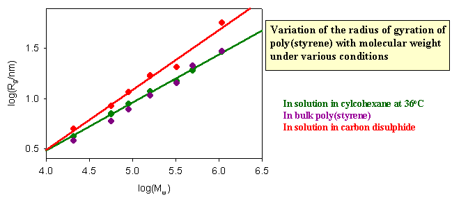
The dimensions of a polymer in solution depend on the nature of the solution. If the nett interaction between distant chain segments is zero (this is the q condition) the conformation should be that of the random flight model. The graph below shows results for different molecular weight poly(styrene)s in cyclohexane, for which the q temperature is 360C. If the radius of gyration is correctly predicted by the random flight model random the slope of the plot of logRg against logMw should be 1/2, which it as at 360C. There is no nett interaction between segments in a q solvent. The free energy of penetration of the polymer by solvent is exactly balanced by the free energy of stretching and these terms cancel at the q point. In a good solvent, however, there is a nett repulsion between segments because the solvent causes the polymer to expand because of the additional favourable enthalpy of interaction between segments and solvent. The radius of gyration then increases. Theoretically and experimentally it is found that <Rg2> is proportional to M6/5 in a good solvent. Carbon disulphide is a good solvent for poly(styrene) and the corresponding plot verifying the change in the behaviour is shown as the red line in the figure below. Also included in the figure are data for the dimensions of poly(styrene) in the bulk amorphous polymer. They are consistent with the random flight model.
The dimensions of a polymer molecule can be determined by x-ray or neutron scattering or, if the polymer is sufficiently large, by light scattering. Since these techniques are also used for studying amphiphile aggregates they are described separately in Scattering Methods.
Gel permeation chromatography (GPC) separates particles according to their effective size in solution. The sample (in solution) is passed through a column of a rigid gel containing pores of a chosen size. Small molecules diffuse in and out of the pores and hence pursue a tortuous route and take a long time to elute through the column. The bigger the polymer molecule in the solution the less easily it will be trapped in one of the pores and the more quickly it will pass through the column. The refractive index (or any suitable physical property) of the solution coming out of the end of the column is monitored and the presence of polymer is easily detected.
The relation between elution time and molecular weight is not linear and depends on a number of factors, one of which is the relation between mean radius and molecular structure of the polymer. The procedure for determining the molecular weight of a polymer is to calibrate the column using known, monodisperse samples with structures as similar as possible to the sample of interest. Both Mn and Mw can be evaluated from the shape of the elution peak.
A useful website is Macrogalleria (a "Cyberwonderland of Polymer Fun"!)
There are many good books on Polymers but they mostly cover far more ground than is needed for the course and so only a small number are listed here. The Colloidal Domain by D.F.Evans and H.Wennerstrom (VCH) covers all aspects of the course. The most appropriate quantitative descriptions are in Polymer Physics by U.W.Gedde, Chapman & Hall. A good, basically qualitative, book on polymers is Giant Molecules by A.Y.Grosberg and A.R.Khokhlov (Academic Press). Other useful books on polymers at this level are Sperling: Introduction to Physical Polymer Science, Billmeyer: Textbook of Polymer Science, Cowie: Introduction to Polymer Science. A good discussion of the thermodynamics of solutions, including polymer solutions, is Ch. 10 of Caldin: Chemical Thermodynamics, but it is out of print and not easy to obtain.