A polymer is generated by joining many monomers together. To show some of the consequences of such a connected structure we use the same simple model that we used to introduce amphiphiles, i.e. chemical groupings with opposing solubility characteristics are represented by different shapes (squares and circles) but those with similar characteristics are represented with different colours but the same shape. The figure below shows one type of circle dissolved in another but with the difference that one sequence of circles is joined to form a polymer. In comparison with free circles, which would form an ideal solution, the movements of the segments of the polymer are restricted and the motion of the polymer molecule in solution is then relatively complex, consisting of changes in conformation with some translational movement of the polymer as a whole. Polymerisation must therefore lead to substantial differences in the solution behaviour. One difference is that any unfavourable interaction of the monomer unit with the solvent is magnified by the large number of such interactions for each polymer molecule. Since dissimilarity generally leads to a positive enthalpy of mixing this means that the polymer only dissolves in a solvent with which its monomer is similar (i.e. circles in circles). The right hand side of the figure shows what happens to the polymer dimensions as the "quality" of the solvent is varied from poor (polymer solubility reduced), through the q condition (where there is no nett effect of solvent on the polymer dimensions) to good. The full range of behaviour illustrated can often occur over a few tens of K or by varying the composition of a mixed solvent over a small composition range.

There are many types of polymer, the simplest being a linear connection of one chemical species to form a homopolymer, of which several examples are given in the panel below. Copolymers involve more than one chemical species and they can be combined in a variety of ways, e.g. alternating, randomly or in blocks. There are also non-linear combinations, e.g. star, comb, dendritic, etc. The selective use of these structural possibilities leads to a wide range of technological applications of polymeric materials.

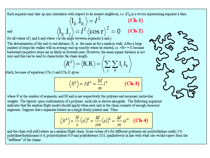
The simplest model of the linked polyer structure is the random flight model. The polymer is assumed to consist of segments which are free to rotate through any angle with respect to adjacent segments. The mean square distance between the ends of the molecule can then be related to the molecular weight and the length of the individual segments as in the panel below. The random flight model only seems unrealistic if one makes the mistake of assuming that a random flight segment is the same as a chemical segment. For each homopolymer the number of chemical segments needed to produce a segment that follows the random flight model varies according to the stiffness of the structure and some values are given for common polymers at the bottom of the panel below.

In a rubber (elastomer) the mobility of the majority of the segments is similar to that in the polymer melt. However, a network of cross-links holds the elastomer together. When the elastomer is stretched there is a decrease in the entropy of the chains between the links. The panel gives a simple treatment of the resulting elasticity.

The factors making a real material elastic are: (i) completely flexible chains (liquid-like motion of the segments to enable rapid sampling of all chain conformations), and (ii) a network of cross-links to hold the whole material together. The network is necessary, otherwise the material would be a melt, and may be achieved in several ways. The figure below shows how such a network can be created by chemical bonds as in the vulcanization of natural rubber by the creation of sulphur links.


One of the consequences of the simple statistical model outlined above is that the force required to stretch the rubber increases with temperature (equation (El-1)). In the panel below a Maxwell relation is derived (equation (Th-2)) which shows that the increase of f with T must be associated with a decrease of S with l, exactly as would be expected from the model of the elasticity derived above.

A number of other observations which fit the general pattern above are that rubber shrinks on heating, whereas other materials expand. Also, when rubber is stretched rapidly it heats up, as can be tested by stretching a rubber band sharply and immediately holding it against the lips. The heating of the rubber band on stretching follows from equation (Th-1). The conditions are approximately adiabatic, i.e. dU = 0. Hence dq = - fdl and heat is given out on stretching.
The thermodynamic properties of a polymer in solution are important in the determination of the molecular weight. Because a polymer is very large in comparison with the solvent molecule the entropy of mixing does not take on the simple form that it has in an ideal solution. As written in the panel below, the mole fractions in the expression for the ideal entropy of mixing must be replaced by volume fractions. There is also a contribution to the free energy of mixing from the enthalpy of mixing of polymer and solvent. Any small enthalpic interaction between a polymer segment and a solvent has to be multpipled by the number of segments. Thus, even small interactions become significant. The calculation of the enthalpy of mixing is the same as used for equations (Sol-2) and (Sol-3) in Amphiphiles. The panel below summarizes the two contributions and substitutes the resulting chemical potential of the solvent into the derivation of the osmotic pressure (see first year lectures on Thermodynamics of Solutions) or new second year lecture course to give the important equation (Fl-2).

Comparison of the ideal and non-ideal expressions for the chemical potential shows that B contains one contribution from the excess entropy of mixing (the 1/2 term in equation (Fl-2)) and one from the excess enthalpy of mixing (the c term). Taking the enthalpy of mixing to be zero leads to a positive value of B, resulting from the positive excess entropy of mixing. The positive excess entropy of mixing creates an additional driving force for diluting the solution with solvent, i.e. a higher osmotic pressure than would be expected from ideal behaviour. The enthalpy of mixing is proportional to the c parameter and is generally positive. A positive c makes mixing less favourable and hence lowers the osmotic pressure below the ideal value. The osmotic pressure appropriate to ideal mixing is obtained by putting B = 0. B is therefore analogous to the second virial coefficent for a gas, for which B is zero when the repulsion arising from the finite size of the molecules is exactly compensated by the van der Waals attraction. For a gas this happens at the Boyle temperature, at which the gas behaves as though it were ideal. This suggests a similar interpretation for the polymer solution. When B is positive the segments behave as though they repel one another because the solvent is forcing them apart (good solvent). When B is negative the positive enthalpy of mixing (c must now be greater than 1/2) makes the solvent a poorer solvent and hence the segments effectively attract one another. At the q point, B is zero and there is no nett interaction between polymer segments. It is at this point that the dimensions of the polymer should conform to the random flight model. Since the entropic contribution to the free energy varies with temperature, the q point can only be at one temperature. However, the quality of a mixed solvent can also be adjusted by varying its composition to give a q point dependent on composition (and temperature).
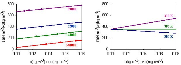
Measurement of osmotic pressure and application of equation (Fl-1) gives a useful method for determining the molecular weight of a polymer. The equation indicates that a plot of P/c against c will give a straight line graph with intercept RT/M2 and a slope proportional to B. Since B is positive for a good solvent the slope of the plot will be positive. Some actual data for different molecular weight samples of neoprene in toluene are shown on the left hand side of the figure below. The virial coefficient is the same for all molecular weights so the slopes are all the same. On the right hand side is shown the effect of varying temperature for a sample of poly(styrene) in cyclohexane, for which the q point is 340C. B is positive at higher temperatures and negative at lower temperatures. Since cyclohexane is a poor solvent for poly(styrene) below 340C one would expect the solubility to be reduced in some way. In fact, the polymer will become insoluble either by a further lowering of the temperature or by an increase in molecular weight.

The molecules in a synthetic polymer sample have a spread of molecular weights. Any measurement of molecular weight therefore gives an average. Different physical techniques measure different averages. Osmotic pressure, being a colligative property, gives the number average molecular weight, i.e.

An alternative method of measuring the molecular weight is to use light scattering (see below), which gives the weight average molecular weight, defined by

It is important point to note that, because polymer samples consist of mixtures of different molecular weight molecules, Mn and Mw are not the same. The extent to which they differ depends on the polydispersity of the sample (the ratio is often used as a measure of the polydispersity; ideally it should be as close to unity as possible).
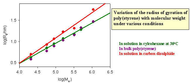
The dimensions of a polymer in solution depend on the nature of the solution. If the nett interaction between distant chain segments is zero (this is the θ condition) the conformation should be that of the random flight model. The graph below shows results for different molecular weight poly(styrene)s in cyclohexane, for which the θ temperature is 340C. If the radius of gyration is correctly predicted by the random flight model random the slope of the plot of logRg against logMw should be 1/2, which it as at 340C. There is no nett interaction between segments in a θ solvent. The free energy of penetration of the polymer by solvent is exactly balanced by the free energy of stretching and these terms cancel at the θ point. In a good solvent, however, there is a nett repulsion between segments because the solvent causes the polymer to expand because of the additional favourable enthalpy of interaction between segments and solvent. The radius of gyration then increases. Theoretically and experimentally it is found that <Rg2> is proportional to M6/5 in a good solvent. Carbon disulphide is a good solvent for poly(styrene) and the corresponding plot verifying the change in the behaviour is shown as the red line in the figure below. Also included in the figure are data for the dimensions of poly(styrene) in the bulk amorphous polymer. They are consistent with the random flight model.

The dimensions of a polymer molecule can be determined by x-ray or neutron scattering or, if the polymer is sufficiently large, by light scattering. Since these techniques are also used for studying amphiphile aggregates they are described separately in Scattering Methods.
Gel permeation chromatography (GPC) separates particles according to their effective size in solution. The sample (in solution) is passed through a column of a rigid gel containing pores of a chosen size. Small molecules diffuse in and out of the pores and hence pursue a tortuous route and take a long time to elute through the column. The bigger the polymer molecule in the solution the less easily it will be trapped in one of the pores and the more quickly it will pass through the column. The refractive index (or any suitable physical property) of the solution coming out of the end of the column is monitored and the presence of polymer is easily detected.
The relation between elution time and molecular weight is not linear and depends on a number of factors, one of which is the relation between mean radius and molecular structure of the polymer. The procedure for determining the molecular weight of a polymer is to calibrate the column using known, monodisperse samples with structures as similar as possible to the sample of interest. Both Mn and Mw can be evaluated from the shape of the elution peak.
The majority of the polymer in the rubber state is liquid-like. When the temperature is lowered the motion of the segments will stop and the system will become amorphous. This often produces a very brittle material (glass). At first sight the transition might be thought not to be simple because some polymers may form some crystalline regions and, in others, different parts may become immobilized at different temperatures. Nevertheless, in many polymers the glass transition occurs over quite a narrow temperature range (less than about 20oC). It is most easily followed by the change in volume of the polymer, the coefficient of expansion being much lower in the glassy state. Dilatometry is used to follow the small volume change.
The temperature of the transition, Tg, is sensitive to the chemical nature of the polymer, the molecular weight and the incorporation of other species as in copolymerization and plasticization. The effect of molecular weight is illustrated by polystyrene. At high molecular weight Tg tends to about 110oC but this drops to about 70oC at Mn = 50000.
The extent to which a polymer will swell when exposed to a smaller molecule will depend on the balance between the elastic energy and the gain in free energy due to solubility. The incorporation of such molecules will generally lower Tg substantially because the small molecules allow the chain segments to have greater freedom. This plasticization is a widely used phenomenona.
An important application of polymers is their use for stabilizing colloidal systems. Polymer is adsorbed on to the surface of the colloidal particle and extends into the solution. When two such coated particles approach, the overlapping polymer chains produce a local polymer concentration higher than that in the surrounding solution. There is then a tendency for solvent to move into the overlap region (just as in the osmotic effect) which generates a repulsive force between the particles. If the range of this repulsive force is sufficiently long it will prevent the particles coagulating because of van der Waals forces.
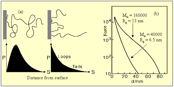
A range of behaviour can be generated according to how the polymer is attached to the surface, the size of the polymer, and the quality of the solvent. Thus a weakly adsorbed polymer has a segment profile which is just a slightly perturbed version of the random flight distribution (see (a) in the figure below), but a strongly attached polymer ((b) in figure below) may produce a high surface density of segments. The latter can be achieved by strong physical forces, as shown in the figure, leading to predominantly loops and tails on the surface, or, more usually, by chemically grafting the polymer on to the surface or by using a block copolymer with one component insoluble, e.g. a poly(ethylene oxide)-poly(propylene oxide) block copolymer (the behaviour then resembles a strongly adsorbed amphiphile). The effect of solvent is crucial. Following the disussion of non-ideal behaviour given above it is clear that a good solvent (positive B) will cause a repulsive interaction between the polymer fragments and hence have a stabilizing effect, but a poor solvent will tend to cause the polymer tails to collapse and hence may lead to an attractive interaction. The range of the repulsive interaction is approximately related to the radius of gyration, as illustrated in (b) below for the forces measured between mica plates for two molecular weights of poly(ethylene oxide) in water.

Two useful websites are Building with Snakes: the Physics of Long-Chain Molecules and the Macrogalleria (a "Cyberwonderland of Polymer Fun"!)
There are many good books on Polymers but they mostly cover far more ground than is needed for the course and so only a small number are listed here. The Colloidal Domain by D.F.Evans and H.Wennerstrom (VCH) covers all aspects of the course. The most appropriate quantitative descriptions are in Polymer Physics by U.W.Gedde, Chapman & Hall. A good, basically qualitative, book on polymers is Giant Molecules by A.Y.Grosberg and A.R.Khokhlov (Academic Press). Other useful books on polymers at this level are Sperling: Introduction to Physical Polymer Science, Billmeyer: Textbook of Polymer Science, Cowie: Introduction to Polymer Science. A good discussion of the thermodynamics of solutions, including polymer solutions, is Ch. 10 of Caldin: Chemical Thermodynamics, but it is out of print and not easy to obtain.