(i) The atomic spectrum of hydrogen. The different series of lines and their relation to the energy level diagram (Grotrian diagram). Interpretation of the levels in terms of the Bohr model of the atom. The determination of the ionization potential from the line spectrum. The spectra of He +, Li2+, Be3+ .
(ii) The nature of the wavefunctions of the hydrogen atom, especially the form of the radial wavefunction. Quantization of angular momentum and the shape of wavefunctions with different values of l. The degeneracy of the angular wavefunctions and space quantization of the angular momentum. The selection rules for l in determining the spectrum.
(iii) Electron spin and the Pauli principle. The atomic spectrum of He. Singlet and triplet series in He.
(iv) Spectra of the alkali metals. The effect on the energy levels of penetration of inner electron shells by the outer electrons. The physical origin of the doublet structure in the alkali spectra. A program that simulates the spectra of the alkali metals and other elements is used below to calculate the spectra of lithium and hydrogen. You can observe the atomic spectrum of sodium in the work for a second year tutorial on electronic spectroscopy.
(v) The coupling of spin and orbital angular momentum. Russell-Saunders coupling of L and S to give the total angular momentum J . Simple term symbols.
(vi) Application of the results to the understanding of the periodic table.
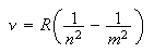
The assignment of the correct values of the quantum numbers to the lines in an atomic spectrum requires an approach of a type that you have not come across before. A given series of lines involves one fixed energy level and a set of levels with a succession of principal quantum numbers, the wavenumber (cm-1) being given by the equation
where n is fixed and m varies. For hydrogen and hydrogen-like atoms it is often easy to guess the starting number of the m series. If the guess is correct a graph of line wavenumber against 1/m2 will give a straight line and the intercept at 1/m2 = 0 (m = ∞) gives the ionization energy of the fixed level. However, it is more difficult to guess the starting value of m for transitions between high values of the principal quantum number and much more difficult to guess for non-hydrogenic atoms. The problem with the latter is that, owing to orbital penetration (the same effect that causes the energy to rise from s to p tod), the energy levels have to be modified by an empirical term, the quantum defect, α. Thus the equation for the lines becomes
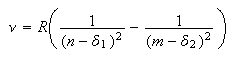
where α has a particular value for each value of l, e.g. all s have the same value of α regardless of n. It is obviously much more difficult to guess the correct value of m when the energy levels depend both on m and the unknown α. It is therefore valuable to have a general means of making a correct assignment of the lines. The applet below indicates how this can be done (click here for information concerning applets; the filenames here are tutorials/atomic/atSpecFit/atSpecFit.jar and tutorials/atomic/atSpecFit/AtSpecFitAppletJ.html). The applet uses these principles and you can use it to answer several of the problems presented below.
The vertical axis represents the wavenumber (could also be frequency) of the lines (in cm-1) and the horizontal axis represents 1/m2. Instead of guessing the appropriate values of m, you draw horizontal lines across the graph at each of the line frequencies and vertical lines at all possible values of 1/m2 where m is an integer. These lines are already drawn in the applet for a series of lines that have been input as data. The correct assignment of the values of m is the set that gives rise to a series of intersections lying on a straight line. The intersections are ringed in the applet. As intially set up, these intersection do not lie on a straight line because the wrong set of m is used. However, without changing the graph we can use the quantum number lever (bottom left) to change to the next set of m. starting at 2 instead of 1 (note that the changes occur in steps as the lever is moved). This produces a good straight line. If you increase the quantum number again the lowest value of m becomes 3 and successive intersections do not lie on a straight line. Thus the correct starting value for this series is m = 2. You would have obtained the same result by plotting a single graph and using a ruler to assess the optimum set of m values. It is important, however, to make the plot on the largest possible scale (for accuracy) and it is sensible to try to guess what the minimum plausible value of the lowest m can be. This can be done for the applet and the optimally adjusted horizontal axis is shown in the version of the applet below. The straight line plot gives the series limit (m = ∞, 1/m2 = 0) as the intercept on the vertical axis. The slope is directly related to the prefactor in the equation for the line frequencies (Rydberg constant). The single plot is therefore usually a complete analysis of the data.
The applet is replotted below with an automatically adjusted horizontal scale. This makes it easier to detect effects of quantum defects and generally gives better visual fits. The data in the initial setting of the applet is for a non-hydrogenic atom. The line frequencies will therefore be affected by the quantum defect. In this particular case, the deviation from linearity when m = 2 cannot be detected visually. However, the line is fitted by least squares (linear regression) in the applet and the residual sum of squares is printed out as the R factor in the upper right hand corner (R here stands for residuals and is not to be confused with the Rydberg constant). The best fit to the data is when R is minimized. A better fit is obtained when the lowest quantum number m = 2 and the quantum defect lever is set to 0.03. You should verify this. This value of the quantum defect is typical of an s series of levels. You will not be asked to determine the quantum defect and the simple linear plot is effective in assigning m values even when the quantum defect is significantly different from an integer.
You can use the applet to fit any set of data. In the blank space at the base of the applet type or paste in the wavenumbers (not the wavelengths) of the lines from lowest to highest and separated by commas. The hydrogen lines in question 3 can be copied and pasted directly. When you are satisfied that your set of numbers is correct, press enter. The applet will now show your plot and you can fit the data as described above. While it is important that you learn to do the plot yourself on a piece of graph paper, you can use the applet to solve all the problems set below.
The simplest books to read are Richards & Scott, The Structure and Spectra of Atoms, Softley, Atomic Spectra and Atkins, Physical Chemistry.
Where the question number is enclosed in a button, e.g. , you can obtain help or comments about the question by clicking it.
The radial wavefunctions for the 2s and 2p orbitals of hydrogen are respectively
where r is the distance of the electron from the nucleus and a0 = 0.05292 nm. Calculate the values of the two wavefunctions for about ten values of r over a suitable range (i.e. until the value of the wavefunction is too small to be interesting). Use these values to calculate the probability of finding the electron at a distance r from the nucleus at the same values of r. Plot both the wavefunctions and the probability. Comment on the differences between the two wavefunctions and on the difference between the two radial probabilities.
2. Do the following test on term symbols, which you should do sufficiently often to produce a good performance (better than 9 right out of 12). An outline of the procedure for determining term symbols is given below. Start the test by clicking the button.
Procedure for determining term symbols.
First note that all complete shells or complete subshells have zero spin and zero orbital angular momentum, so they may be neglected. Then determine the possible positive values of the total orbital angular momentum (L) by vector addition of the individual orbital angular momenta (l) of the remaining electrons. Each value is given the appropriate letter symbol and these are the basic states.
Now determine the possible positive values of the total electron spin angular momentum (S) by addition of the individual spins. For a given total spin the number of allowed orientations is 2S+1 and is called the multiplicity.
Provided that the electrons you are considering are not in the same subshell (this is the case for all the configurations in this question) you combine each value of the multiplicity with each orbital angular momentum state, e.g. 2P.
For each such state calculate the possible positive values of the total angular momentum (J) obtained by combining L and S for that state. Each value obtained is attached as a subscript to the starting state. There will be a separate substate for each value of J obtained.
The emission spectrum of the hydrogen atom contains a series of lines of wavenumber (cm-1) 5333, 7801, 9142, 9950, 10475. Use a graphical procedure to determine the ionization energy from the lowest level in the series. Identify the principal quantum number of this level and calculate a value for the Rydberg constant (the applet will give you the most accurate answer). Verify that the quantum defect is zero.
Use your value of the Rydberg constant (this is determined from the ionization energy; it is nothing to do with the R factor in the applet) to identify the five lines shown in the visible region of the hydrogen discharge spectrum shown in the applet below. (the filenames here are tutorials/atomic/atomic/atomic.jar and tutorials/atomic/atomic/AtSpectraAppletJ.html). (If the spectrum does not come out well, press the Refresh button in the View menu).

The emission spectrum of lithium, shown as a discharge spectrum in the pictures below (if the spectrum does not come out well, press the Refresh button in the View menu) contains three series of lines. The wavelengths of the first series are 671, 323, 274, 256, and 248 nm. Use the applet to estimate the energy required to ionize lithium from the lowest level involved in this series (don't forget to convert wavelengths to wavenumbers).
The other two series are at wavelengths of (a) 813, 497, 427, 399 nm and (b) 610, 460, 413, 391 nm. Use the applet at the start to show that these terminate in a common level (do this with and without the use of the quantum defect lever). Determine the precise ionization energy of this level and by comparison with the first series assign the likely quantum numbers of this level. What are the terms symbols for each series?
Identify the wavelengths of the two strongest lines in the visible spectrum that are not members of the three series above. Give plausible explanations of the origins of these three lines.

5. Write down the possible term symbols for atoms with the electron configurations (i) 2s2 (ii) 2s3 s (iii) 2p3d (iv) 2p3p.
Write down the possible term symbols for an atom with the electron configuration 2p2.
7. The following two statements are wrong in one or more respects. Discuss the statements carefully, explain the errors involved, and provide an accurate version of each statement.
(a) The main absorption lines in the atomic spectrum of sodium vapour are a doublet corresponding to a transition between two doublet 2 P states.
(b) In a He discharge lamp a series of lines are observed corresponding to transitions from 3P to 1 S states.
8. Two series of lines in the discharge spectrum of helium result from transitions from the first excited 1S and the ground 3S. The wavelengths of the lines in each series are (a) 1S : 501.5, 396.4, 361.3, 344.7 nm and (b) 3S: 388.8, 318.7, 294.5 nm.
Use the applet at the start to determine the ionization energies from these two states and hence determine the energy difference between these two states.